Why maximum likelihood-based training may lead to the generation of unrealistic samples
Generative models specify procedures allowing us to produce data samples, e.g., images, texts, user preferences, etc. These models are central to unsupervised learning, and popular examples include mixture models [1], mixed membership models such as latent Dirichlet allocation [2] and probabilistic matrix factorization [3], variational autoencoders [4], just to name a few. In this post, we discuss the behavior of maximum likelihood-based training, and we show that this procedure may result in models that can produce unrealistic samples, i.e., which are unlikely under the real data distribution.
Setting
We are typically given a set of observations (e.g., images) x_1, \ldots, x_n , and our goal is to come up with a model that would allow us to generate samples that look like our observations. To this end, a common approach consists in positing a parametric model p_\theta(x) and estimating it from our data. A predominant framework in this context is maximum likelihood (ML) estimation. The idea is to find the value of the parameters \theta that are most likely to have generated the observations, by maximizing the log-likelihood function:
\mathcal{L}(x;\theta) = \sum_{i=1}^{n}\log{p_\theta(x_i)}
Note that in practice, the likelihood will often be intractable, and we will need to resort to some approximation methods before proceeding with parameter estimation. For the purpose of this post, however, we do not have to worry about that.
Behavior of the ML estimation and its impact on the generated samples
To gain some insights into the behavior of ML-based training, we rely on the general fact that, maximizing the log-likelihood function is equivalent to minimizing the Kullback-Leibler (KL) divergence between the empirical data distribution \tilde{q}(x) and our model distribution p_\theta(x):
KL(\tilde{q}||p_\theta) = \mathbb{E}_{\tilde{q}}\left[\log{\frac{\tilde{q}(x)}{p_\theta(x)}}\right] = -\frac{1}{n}\sum_i\log{p_\theta(x_i) \; -\; \mathbb{H}(\tilde{q})}
where \tilde{q}(x) = \frac{1}{n} \sum_{i=1}^{n} \delta(x\!-\! x_i) , and \mathbb{H} (\tilde{q}) stands for the entropy of the empirical distribution, which is constant and does not affect learning. Note that the likelihood term in the above expression also corresponds to a Monte Carlo estimator of \mathbb{E}_q [p_\theta(x)] where q(x) is the real data distribution. Hence asymptotically, ML estimation amounts to minimizing KL(q||p_\theta). For simplicity, we assume that the above KL is well defined, although in practice it may not always be the case (e.g., if p_\theta(x) is zero in regions where q(x) is non-zero).
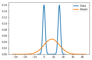
From the definition of the Kullback-Leibler divergence, notice that a very small p in regions of the x space where q is non-negligible will cause the KL to be large. Hence, minimizing the above KL would typically lead to a distribution p_\theta(x) that stretches to cover all q(x) to the expense of putting non-negligible probability mass in regions of the input space where q(x) is close or even equal to zero. This phenomenon is commonly referred to as the zero-avoiding behavior in the literature [5, 6], and it can be easily illustrated by trying to fit a unimodal distribution to observations arising from a multimodal distribution. Figure 1 provides such an illustration. Here our observations come from a 2-component, \mathcal{N}(0,1) and \mathcal{N}(16,1), Gaussian mixture model (blue curve), and p_\theta(x) is a Gaussian with unknown mean \mu and variance \sigma^2, i.e., \theta = \{\mu,\sigma\}. Fitting our model to the data yields the orange distribution with the ML estimates \mu^{*} = 8, \sigma^{*} = 8.06. The latter distribution averaged over the modes of our data distribution, and as a result, its mode falls in a region of our input space where the data distribution q(x) is very small. Clearly most of the samples from the resulting model would not look like our observations.

The undesirable behavior of ML-based training observed on this toy example is a consequence of the under-specification of p_\theta(x), and we would perfectly fit our data distribution by assuming p to be a member of the two-component Gaussian mixture family. In practice however, the real data distribution will often be unknown to us, and the same phenomenon may occur whenever we deal with data following some complex distribution (e.g., images, texts, etc.), and we specify a family of models that is not rich/flexible enough to approximate well the underlying data distribution.
Discussion
Our example sheds some light on why some popular generative models (e.g., variational autoencoder VAE [4]), which usually rely on ML-based training, often lead to blurriness in the generated samples (in the case of image data) or even to unrealistic samples in some situations. The above results also provide some useful insights on how we can cope with the problem of unrealistic sample generation.
One possibility is to specify a highly flexible family of models p_\theta(x) and hope that it has enough capacity to fit well the real data distribution. For instance, in our earlier example we can recover the real data distribution by specifying a richer model, e.g., a Gaussian mixture model with two or more components. However, this may come at the cost of making ML-based training even more challenging.
Another natural remedy to unrealistic sample generation is to consider other discrepancy measures that do not exhibit the zero-avoiding behavior [7, 8, 9], such as Wasserstein distance, Jensen-Shannon divergence, reverse KL, i.e., KL(p_\theta||q), etc. However, these measures usually pose other difficulties and in general require some adversarial learning, which is known to be a highly unstable training procedure. In particular, one issue we may encounter with some of these alternatives is mode collapse, i.e., the trained model captures only one mode of the data distribution. That said stabilizing adversarial learning and addressing the mode collapse issue are active research topics, and important progress is being made.


